Written By Sophanith Dith
Last Updated April 29, 2026
Applies to Microsoft Excel 365 (Windows only)
The easiest way to understand how to find average in Excel is to use the AVERAGE function. This function adds numbers together, counts how many numeric values are included, and returns the average result automatically.
Learning how to use the AVERAGE function in Excel is useful when you want to analyze scores, sales, expenses, hours worked, ratings, or any list of numbers. Instead of adding values manually and dividing by the count, Excel does the calculation for you with one formula.
Before using it in real examples, it helps to understand exactly what the function does.
What the AVERAGE Function Does
The AVERAGE function calculates the average, also called the arithmetic mean, of a group of numbers. In simple terms, it finds the typical value from a list of numeric values.
For example, in Sales_Report.xlsx, suppose cells B2:B6 contain daily sales amounts. You can use the AVERAGE function to find the average daily sales for that period.
The function is useful when you need to answer questions like:
- What is the average test score?
- What is the average monthly expense?
- What is the average sales amount?
- What is the average number of hours worked?
Important Note:
The result returned by the formula is a number. Excel ignores blank cells in the selected range, but it includes cells that contain zero. This difference matters because a blank cell means “no value,” while zero is treated as an actual number.
If you are still learning how formulas work in Excel, you may also want to review formulas and functions in Excel to understand the difference between typing a formula and using a built-in function.
Now that you know what the function does, the next step is learning the correct formula structure.
AVERAGE Function Syntax
The syntax tells Excel which numbers to average. The AVERAGE function can use individual numbers, cell references, or full cell ranges.
The basic syntax is:
=AVERAGE(number1, [number2], ...)
Microsoft’s AVERAGE function guide also explains that the function returns the arithmetic mean of its arguments.
Here is what each part means:
| Argument | Required? | Meaning |
|---|---|---|
| number1 | Yes | The first number, cell, or range you want to average |
| [number2] | Optional | Additional numbers, cells, or ranges to include |
For most beginner worksheets, you will usually use a range like this:
=AVERAGE(B2:B10)
This tells Excel to find the average of all numeric values from B2 through B10. In most beginner worksheets, number1 is usually a cell range, such as B2:B10.
You can also average separate cells:
=AVERAGE(B2,D2,F2)
This averages only the selected cells, not the cells between them.
The AVERAGE function supports numbers, cell references, and ranges. It is not case-sensitive, so =average(B2:B10) still works, but using uppercase function names is easier to read.
Once the syntax is clear, the easiest way to learn is with a small worksheet example.
How to Find Average in Excel with a Basic Example
A simple example makes it easier to see how the average formula in Excel works. Imagine you have a short list of test scores and want to find the average score.
In Employee_List.xlsx, suppose your worksheet looks like this:
| Cell | Value |
|---|---|
| B1 | Score |
| B2 | 80 |
| B3 | 90 |
| B4 | 75 |
| B5 | 85 |
| B6 | 70 |
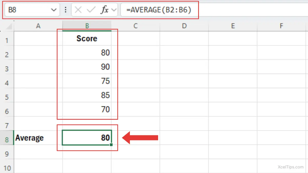
To find the average score, enter this formula in B8:
=AVERAGE(B2:B6)
Excel returns 80, which is the average score.
This result appears because Excel adds the numbers together:
80 + 90 + 75 + 85 + 70 = 400
Then it divides by the number of values:
400 / 5 = 80
This is the most common way to find average in Excel because it is short, clear, and easy to check.
After you understand the basic version, you can apply the same function to real business, budget, and tracking examples.
Practical Examples of the AVERAGE Function in Excel
The AVERAGE function is useful in many everyday worksheets. The formula stays simple, but the purpose changes depending on the data you are analyzing.
Example 1: Find Average Monthly Expenses
In Budget.xlsx, suppose cells B2:B7 contain expenses for January through June.
| Month | Expense |
|---|---|
| January | 1200 |
| February | 1350 |
| March | 1100 |
| April | 1400 |
| May | 1250 |
| June | 1350 |
Use this formula:
=AVERAGE(B2:B7)
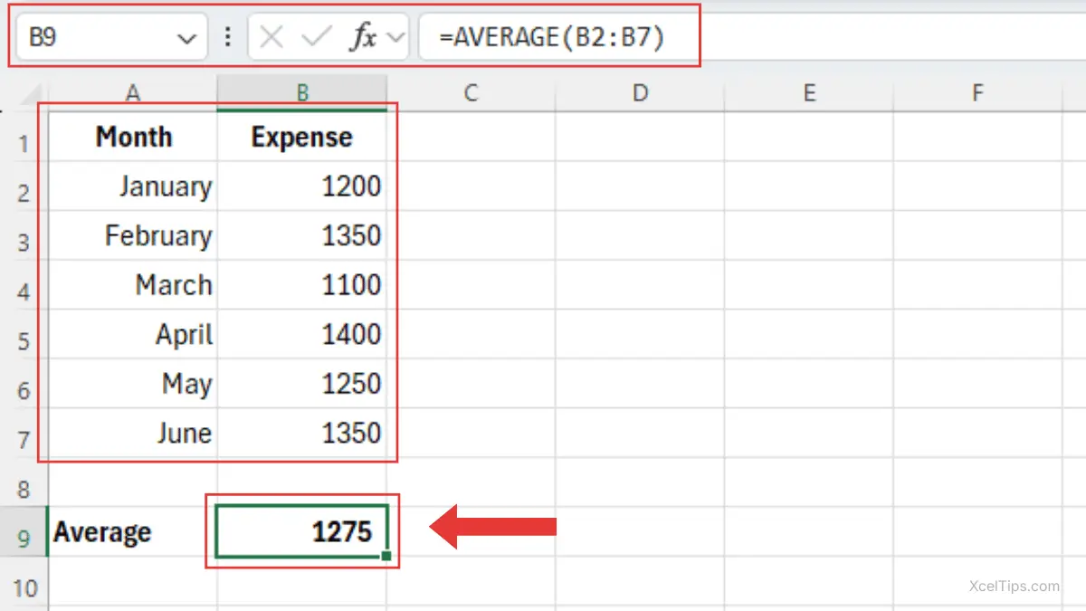
Excel returns 1,275. This is the average monthly expense, which helps you understand your typical spending instead of looking at each month separately.
Example 2: Calculate Average Sales
In Sales_Report.xlsx, suppose cells C2:C8 contain sales totals for one week. To calculate the average daily sales, use:
=AVERAGE(C2:C8)
This helps you see the normal daily sales level, which can be more useful than focusing only on the highest or lowest day.
If your next step is adding all sales before comparing the average, you can review how to use the SUM function in Excel. SUM calculates the total, while AVERAGE calculates the typical value.
Example 3: Average Hours Worked
In an employee tracking sheet, suppose D2:D11 contains weekly hours worked by team members.
=AVERAGE(D2:D11)
This formula returns the average number of hours worked. It helps you see the typical number of hours worked without calculating the average manually.
Example 4: Average Non-Adjacent Cells
Sometimes the values you want to average are not next to each other. For example, if quarterly results are in B2, D2, F2, and H2, use:
=AVERAGE(B2,D2,F2,H2)
This is useful when your worksheet has other columns between the values you want to include.
If you need to copy the formula across several rows, a quick fill method can save time. For a separate productivity lesson, see how to use AutoFill in Excel.
These examples cover the most common uses, but beginners often run into a few predictable mistakes.
Common Mistakes When Using the AVERAGE Function
The AVERAGE function is simple, but small worksheet issues can change the result. Knowing these mistakes will help you use the formula more accurately.
1. Including the Wrong Range
A common mistake is selecting too many or too few cells.
Wrong example:
=AVERAGE(B2:B100)
If your actual data only goes to B10, this may include extra cells you did not intend to average.
Correct example:
=AVERAGE(B2:B10)
Always check that the selected range matches your real data. Extra blank cells usually do not change the result, but selecting the wrong range can include old numbers, hidden values, or cells you did not mean to average.
2. Confusing Blank Cells and Zero Values
Excel ignores blank cells, but it includes zero values.
For example:
=AVERAGE(B2:B8)
If one cell is blank, Excel ignores it. If one cell contains 0, Excel includes it in the calculation. This can lower the average.
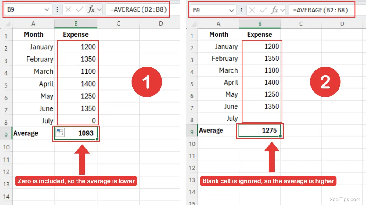
Beginner Tip:
In a selected range, the AVERAGE function ignores blank cells and text entries. It only includes numeric values. However, a cell that contains 0 is counted as a real number, so it can lower the average.
The table below shows how the AVERAGE function treats different types of cell content when they are included in the selected range.
| Cell content | How AVERAGE treats it |
|---|---|
| Blank cell | Ignored |
Text such as N/A or No data | Ignored |
0 | Included as a number |
Number such as 1200 | Included as a number |
3. Averaging Numbers Stored as Text
Sometimes numbers look correct but are stored as text. When those values are inside a selected range, Excel may ignore them instead of treating them as real numbers.
To fix this, convert the text values into real numbers before using the AVERAGE formula.
4. Typing the Formula Without the Equal Sign
Every Excel formula must begin with an equal sign.
Wrong:
AVERAGE(B2:B10)
Correct:
=AVERAGE(B2:B10)
Without the equal sign, Excel treats the entry as plain text instead of a formula.
5. Including Labels in the Formula Range
If your column header is included in the range, Excel usually ignores the text label, but it is still cleaner to select only the numbers.
Better formula:
=AVERAGE(B2:B10)
Instead of:
=AVERAGE(B1:B10)
Clean ranges make formulas easier to read and troubleshoot.
Once you can avoid these common mistakes, it becomes easier to understand how AVERAGE connects to other basic Excel formulas.
Related Formulas
The AVERAGE function is often used beside other summary formulas, especially when you want to compare totals, counts, lowest values, and highest values. These formulas answer different questions about the same set of numbers.
| Formula | What It Does | Difference from AVERAGE |
|---|---|---|
| SUM | Adds numbers together | Returns the total, not the average |
| COUNT | Counts numeric cells | Counts values but does not calculate an average |
| MIN | Finds the smallest number | Shows the lowest value only |
| MAX | Finds the largest number | Shows the highest value only |
For example, if you are reviewing sales data, SUM tells you total sales, AVERAGE tells you typical sales, MIN tells you the lowest sales value, and MAX tells you the highest sales value.
These related formulas are helpful, but the main purpose of this article is understanding how to average in Excel with the AVERAGE function.
Now you can practice the formula with a few simple exercises.
Quick Practice
Use XcelTips_Practice.xlsx to try to practice the AVERAGE function yourself. These exercises are short and focused on the formula.
- In cells
B2:B6, enter five test scores. InB8, enter:
=AVERAGE(B2:B6)
- In cells
C2:C7, enter monthly expense amounts. InC9, calculate the average monthly expense. - In cells
D2:D6, enter sales values. Change one value to0, then compare how the average changes.
These small practice tasks will help you understand how the formula reacts to different numbers, blanks, and zero values.
Before finishing, here are answers to common beginner questions.
Frequently Asked Questions (FAQs)
What is the formula to find average in Excel?
The basic formula is:
=AVERAGE(range)
For example:
=AVERAGE(B2:B10)
This finds the average of the numbers in cells B2 through B10.
How do I use the average function in Excel?
To use the average function in Excel, type =AVERAGE(, select the cells you want to average, close the parenthesis, and press Enter.
Example:
=AVERAGE(C2:C8)
Does Excel include blank cells in an average?
No. Excel ignores blank cells when calculating an average. However, Excel does include cells that contain zero.
Why is my AVERAGE formula not working?
Common reasons include missing the equal sign, selecting the wrong range, using numbers stored as text, or including cells that do not contain valid numbers.
Can I average cells that are not next to each other?
Yes. Separate each cell reference with a comma:
=AVERAGE(B2,D2,F2)
This averages only those specific cells.
Conclusion
Learning how to find average in Excel is one of the most useful first steps in working with formulas. The AVERAGE function helps you quickly calculate a typical value from scores, sales, expenses, hours, or any other numeric data.
The key is to choose the correct range, remember that blanks and zeros are treated differently, and check that your values are real numbers. After practicing AVERAGE, you may want to continue with a related formula such as how to use the SUM function in Excel or follow the beginner learning path to build your skills in the right order.