How to Hide Rows in Excel Without Deleting Your Data

Written By Sophanith Dith
Last Updated May 06, 2026
Applies to Microsoft Excel 365 (Windows only)
Part of the Beginner Learning Path
Module 2 Working with Data
Lesson 9 of 22

Sometimes your worksheet includes rows you do not need to show all the time. You may have extra notes, blank rows, helper data, old information, or details that make the worksheet harder to read. Learning how to hide rows in Excel helps you keep the data in the file while making the worksheet look cleaner.

Hiding a row does not delete anything. It only removes the row from view. The data, formulas, and formatting stay in the workbook, and you can show the row again later when needed.

This tutorial will show you several beginner-friendly ways to hide one row, multiple rows, non-adjacent rows, and unused rows in Excel.

Quick Answer:
To hide rows in Excel, select the row number or row numbers you want to hide, right-click the selected row header, and choose Hide. You can also use the shortcut Ctrl + 9. Hidden rows are not deleted; they are only removed from view.

Before following the detailed steps, use this quick reference to choose the method that matches what you want to hide.

Quick Reference

Here is a quick overview before you follow the full steps.

• To hide one row, right-click the row number and choose Hide.
• To hide multiple rows together, select the row numbers first, then choose Hide.
• To hide non-adjacent rows, hold Ctrl while selecting row numbers.
• The shortcut to hide rows in Excel is Ctrl + 9.
• You can also use Home tab → Cells group → Format → Hide & Unhide → Hide Rows.
• Hidden rows stay in the workbook and can be shown again later.

Before using the Hide command, it is important to understand what hiding a row actually does to your worksheet.

What Happens When You Hide Rows in Excel?

Before you hide anything, it helps to understand what Excel is actually doing. Hiding rows changes the worksheet view, but it does not remove the row from the file. This is different from deleting a row.

When you hide a row, Excel keeps the row’s data in place. The row becomes invisible, and the row numbers on the left side skip over the hidden row number. For example, if row 6 is hidden, you may see row 5 followed by row 7.

This is useful when you want to temporarily clean up a worksheet without removing information. For example, you might hide rows that contain notes, helper calculations, or old data that you do not need to see while presenting the worksheet.

If you are trying to permanently remove rows, use the separate guide on how to delete rows in Excel instead. Hiding is for temporarily changing what you see. Deleting removes the row from the worksheet.

Once you understand that hiding does not delete data, you can start with the easiest method: using the row number and right-click menu.

How to Hide a Row in Excel with the Mouse

The simplest way to hide a row in Excel is to use the row number on the left side of the worksheet. This method is easy for beginners because you can see exactly which row you are working with.

Hide One Row

Follow these steps to hide a row in Excel.

1. Click the row number on the left side of the worksheet to select the entire row.
2. Right-click the selected row number.
3. Choose Hide from the shortcut menu.

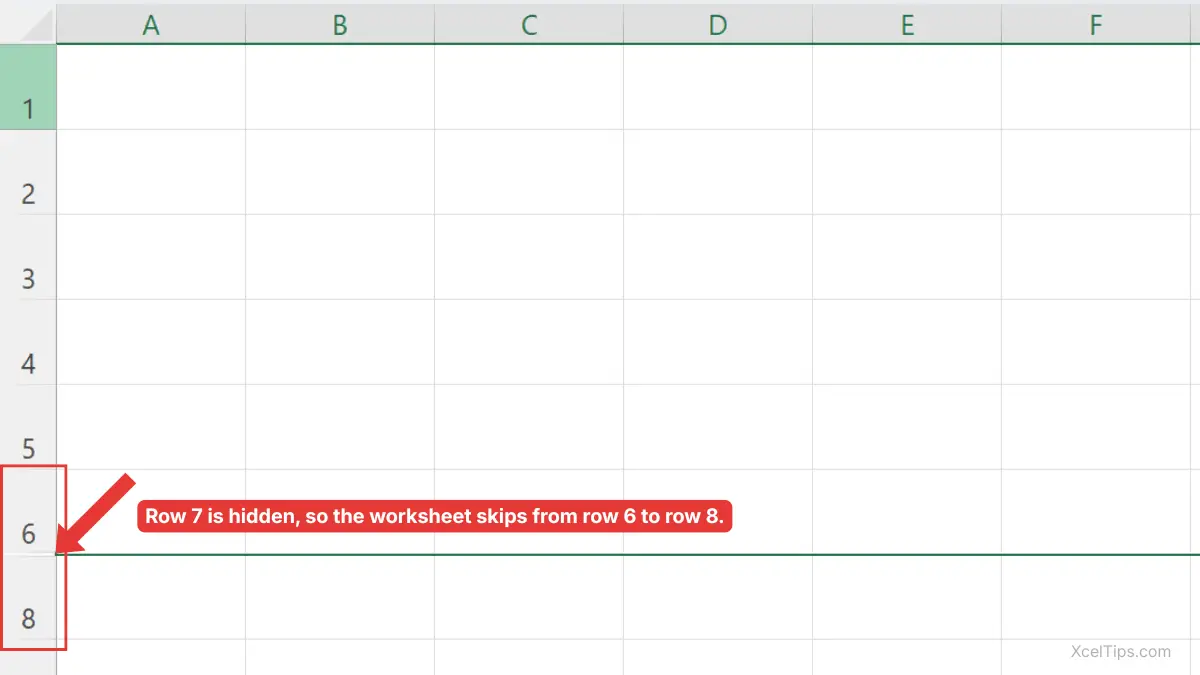
Excel hides the selected row from view.

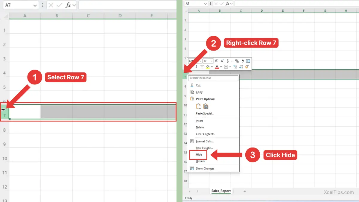
For example, suppose row 7 contains old notes that you do not want to show in a sales list. Click row number 7, right-click it, and choose Hide. Excel hides row 7, but the information remains in the workbook.

The image below shows the result after row 7 is hidden.

Beginner Tip:
Always click the row number, not just a cell inside the row. Clicking the row number selects the full row, which makes the Hide command easier to understand.

After learning how to hide one row, the next step is hiding several rows at the same time.

Hide Multiple Adjacent Rows

Sometimes the rows you want to hide are next to each other. For example, you may want to hide rows 10 to 15 because they contain extra details that are not needed in the main view.

This method is useful when you want to hide rows in Excel as one continuous block.

First select the full group of rows, then use the Hide command.

1. Click and hold the first row number you want to hide, then drag down to the last row number.
2. Release the mouse button when all rows are selected.
3. Right-click any selected row number.
4. Choose Hide.

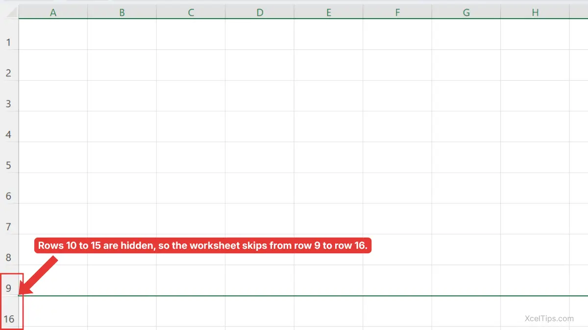
Excel hides all selected rows at the same time.

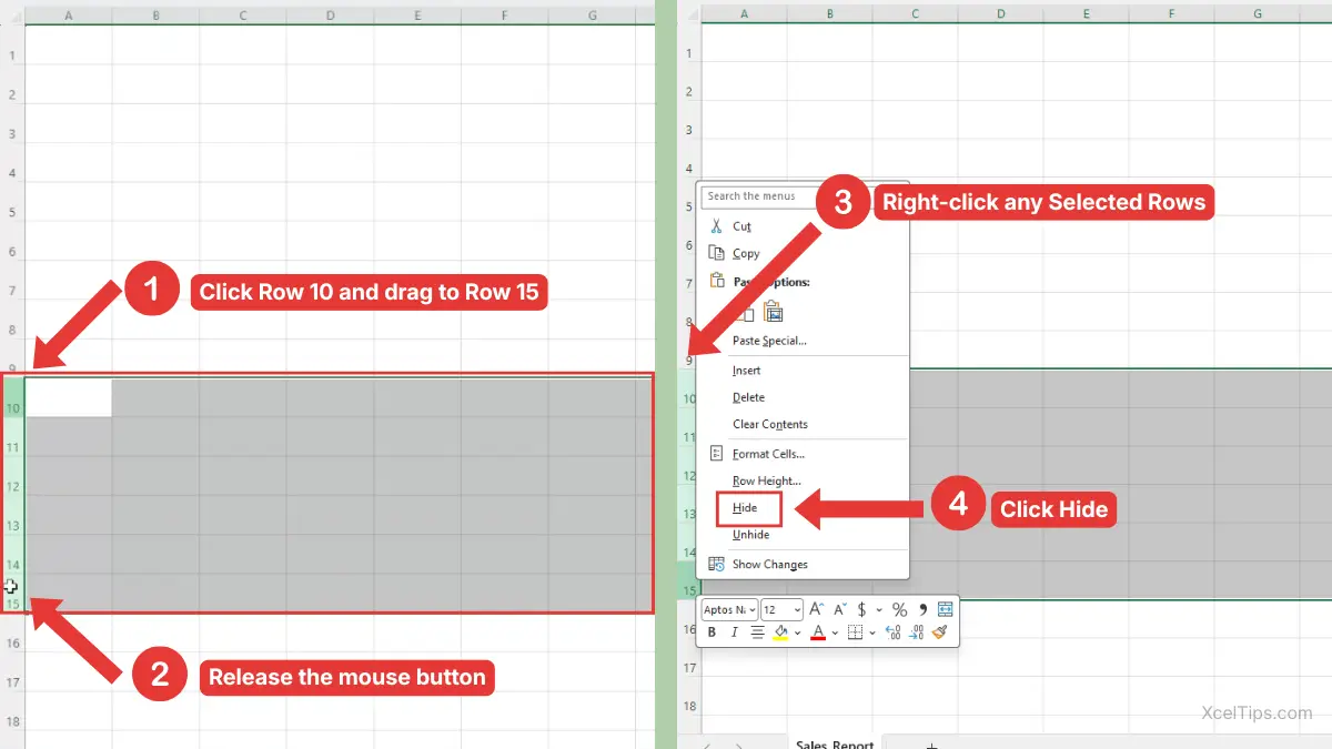
For example, suppose rows 10 to 15 contain extra product notes. Select row numbers 10 through 15, right-click one of the selected row numbers, and choose Hide. Excel hides the entire block.

The image below shows the result: the worksheet skips from row 9 to row 16.

If selecting rows still feels new, you can review the related guide on how to select rows in Excel before practicing this method.

Beginner Warning:
Do not drag across the cells inside the worksheet if your goal is to hide full rows. Select the row numbers on the left instead.

Sometimes the rows you want to hide are not next to each other, so you need a slightly different selection method.

Hide Non-Adjacent Rows

Non-adjacent rows are rows that are not next to each other. For example, you may want to hide rows 1, 6, and 9, but keep all the rows between them visible.

This is useful when you want to hide only certain rows while leaving the rows between them visible.

To select separate rows, use the Ctrl key while clicking row numbers.

1. Click the first row number you want to hide.
2. Hold Ctrl on your keyboard.
3. While holding Ctrl, click each additional row number you want to hide.
4. Release Ctrl after all rows are selected.
5. Right-click one of the selected row numbers.
6. Choose Hide.

Excel hides all selected non-adjacent rows.

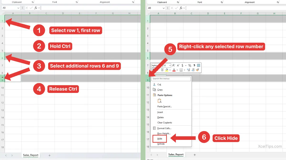
For example, suppose rows 1, 6, and 9 are blank inside a sales worksheet. Hold Ctrl, click row numbers 1, 6, and 9, then right-click and choose Hide. Excel hides those selected rows while keeping the rows between them visible.

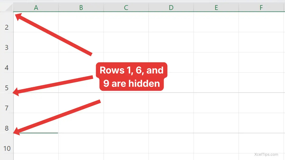
The image below shows the result: rows 1, 6, and 9 are hidden, while the other rows remain visible.

Beginner Tip:
Keep holding Ctrl until you finish selecting all the separate row numbers. If you release it too early and click another row, Excel may replace your selection.

If you plan to hide rows often, the keyboard shortcut can make the process much faster.

Shortcut to Hide Rows in Excel

The fastest shortcut to hide rows in Excel is Ctrl + 9. This shortcut is useful when you repeat the same action often and want to avoid opening the right-click menu.

The shortcut works for one row, adjacent rows, or non-adjacent rows. The only difference is that you must select the row or rows first, then press Ctrl + 9.

Use this method when you already know which row should be hidden.

1. Select the row number you want to hide.
2. Press Ctrl + 9.
3. Excel hides the selected row.

For example, if row 8 contains temporary notes, click row number 8 and press Ctrl + 9. Excel hides row 8 immediately.

You can also select a cell in the row and press Ctrl + 9, but beginners should select the row number first. That makes it clearer which row will be hidden.

To hide multiple rows with the shortcut, select the adjacent or non-adjacent row numbers first, then press Ctrl + 9. Excel hides all selected rows at the same time.

This table summarizes the main shortcut covered in this lesson.

Action	Shortcut
Select the full row of the active cell	Shift + Space
Hide the selected row or rows	Ctrl + 9

For a faster workflow, click a cell in the row, press Shift + Space to select the full row, then press Ctrl + 9 to hide it.

The shortcut is fast, but the Ribbon method is helpful when you prefer to find commands visually.

Hide Rows from the Ribbon

The Ribbon method is useful if you prefer clicking commands instead of using the right-click menu or keyboard shortcuts. It also helps beginners find the visibility commands in the Ribbon.

This method uses the Home tab and the Format menu. The Ribbon method also works for one row, adjacent rows, or non-adjacent rows. Select the row or rows first, then use the same Hide Rows command.

Start by selecting a row you want to hide.

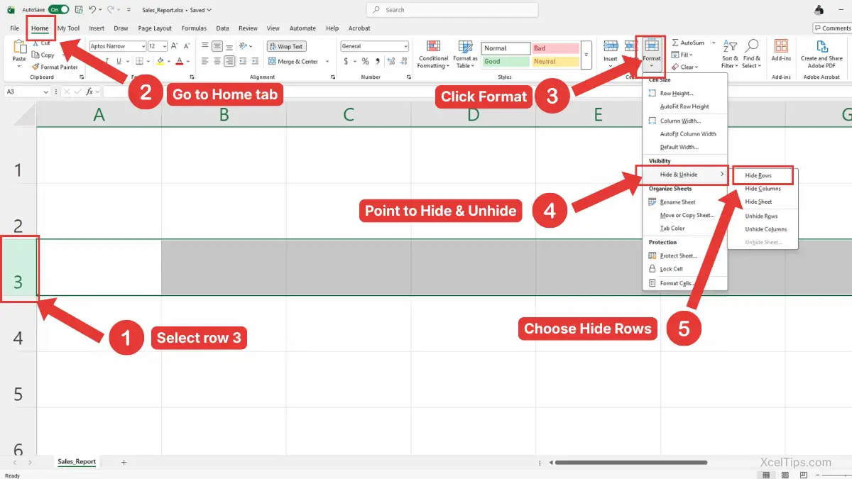
1. Select the row number you want to hide.
2. Go to the Home tab.
3. In the Cells group, click Format.
4. Point to Hide & Unhide.
5. Choose Hide Rows.

Excel hides the selected row.

This method is especially useful if you are teaching someone else or following a visual tutorial. It takes more clicks than the shortcut, but it is clear and easy to follow.

To hide multiple rows from the Ribbon, select all the row numbers you want to hide before opening the Format menu. The same Hide Rows command will hide every selected row.

Beginner Tip:
The Hide Rows command only works as expected when a row or a cell in the row is selected. If nothing is selected, Excel may not hide the row you intended.

For official instructions, you can also review Microsoft’s guide to hiding and showing rows or columns in Excel.

Now that you know the main methods, it helps to see when hiding rows is actually useful in real worksheets.

Practical Examples of When to Hide Rows in Excel

Hiding rows is most useful when you want a cleaner worksheet without removing information. Beginners often use it for reports, lists, notes, and temporary data.

Here are a few common situations where hiding rows makes sense.

Hide Blank Rows in Excel

You may have blank rows inside a list that make the worksheet look uneven. If there are only a few blank rows, you can select those row numbers and hide them.

For example, suppose rows 9 and 14 are blank inside a small customer list. Hold Ctrl, click row numbers 9 and 14, right-click one of them, and choose Hide.

This can make the list easier to read, but it does not actually remove the blank rows. If your goal is to clean the data permanently, deleting or filtering may be better.

Hide Unused Rows in Excel

Sometimes a worksheet only uses a small area, such as columns A to E and rows 1 to 30. If you want the worksheet to look cleaner, you may choose to hide unused rows below the working area.

For example, if your useful data ends at row 30, you can select rows 31 and below, then hide them. This makes the visible sheet feel more focused.

Be careful with this method. Hiding too many unused rows can make navigation confusing for beginners, especially if they later forget rows were hidden.

Hide Helper Rows

Some worksheets include helper rows used for notes, checks, or extra calculations. You may want those rows to stay in the workbook but not appear in the main view.

For example, if rows 20 to 22 contain internal notes for a report, you can hide those rows before sharing or presenting the worksheet.

If you also work with columns, the related skill is how to hide columns in Excel. The idea is similar, but the selection happens from column letters instead of row numbers.

Hiding rows is useful, but you also need to recognize when rows are already hidden.

How to Recognize Hidden Rows in Excel

Hidden rows can confuse beginners because the worksheet may look like rows are missing. Excel gives you a few visual clues when rows are hidden.

The most common clue is skipped row numbers. For example, if you see row 5 followed by row 9, rows 6 to 8 are probably hidden.

You may also notice a small gap or double line between the visible row numbers. This shows where hidden rows are located.

Suppose your worksheet shows these row numbers:

Visible Row Numbers	What It Means
1, 2, 3, 4, 5, 6	No obvious hidden rows in this section
1, 2, 3, 7, 8	Rows 4 to 6 may be hidden
10, 11, 15, 16	Rows 12 to 14 may be hidden

This is important because hidden rows can still affect formulas, totals, and worksheet structure. The data is still there, even though you cannot see it.

Because hidden rows are easy to overlook, it is worth learning the most common mistakes before using this feature often.

Common Mistakes When Hiding Rows

Hiding rows is simple, but beginners can run into problems when they forget what hiding actually does. Most mistakes happen because hidden rows look like missing rows.

Use this table to avoid common issues.

Mistake	Why It Happens	Better Habit
Hiding instead of deleting	You want the data removed permanently	Use delete when the row is no longer needed
Forgetting rows are hidden	Row numbers are skipped but easy to miss	Check row numbers before editing or sharing
Selecting cells instead of row numbers	Only part of the worksheet appears selected	Click the row number to select the full row
Hiding too many unused rows	The worksheet becomes harder to navigate	Hide only rows that improve readability
Thinking hidden data is gone	Hidden rows are invisible	Remember the data remains in the workbook

The most important point is simple: hidden rows are still part of your worksheet. They are just not visible.

If you need to bring rows back later, that belongs in the next lesson on how to unhide rows in Excel.

The best way to remember this skill is to try it in a small practice worksheet.

Quick Practice

Try this short practice in a blank worksheet or a sample file such as Xceltips_Practice.xlsx.

1. Type sample labels in cells A1 to A8.
2. Click row number 4.
3. Right-click row 4 and choose Hide.
4. Notice that the row numbers skip from 3 to 5.
5. Select rows 6 to 8.
6. Press Ctrl + 9.
7. Look at the row numbers again and identify which rows are hidden.

This practice helps you understand both the mouse method and the shortcut method.

Before you finish, here are the most important points to remember about hiding rows in Excel.

Key Takeaways

• Hiding rows removes rows from view but does not delete the data.
• The easiest way to hide a row in Excel is to right-click the row number and choose Hide.
• To hide multiple rows, select the row numbers first, then use Hide.
• The shortcut to hide rows in Excel is Ctrl + 9.
• Hidden rows can be identified by skipped row numbers.
• Use hiding when you want a cleaner layout, not when you want to permanently remove data.

Frequently Asked Questions (FAQs)

Here are answers to common beginner questions about hiding rows in Excel.

How do I hide rows in Excel?

Select the row number or row numbers you want to hide, right-click the selected row header, and choose Hide. You can also press Ctrl + 9 after selecting the row.

How do I hide a row in Excel?

Click the row number on the left side of the worksheet, right-click the selected row number, and choose Hide. This hides the full row from view.

What is the shortcut to hide rows in Excel?

The shortcut to hide rows in Excel is Ctrl + 9. Select the row or rows first, then press the shortcut.

Does hiding a row delete the data?

No. Hiding a row does not delete the data. The row is only removed from view, and the information remains in the workbook.

Can I hide multiple rows at once?

Yes. Select multiple row numbers, right-click one of the selected row numbers, and choose Hide. You can select adjacent rows by dragging or non-adjacent rows by holding Ctrl while clicking row numbers.

Why are some row numbers missing in Excel?

Missing row numbers usually mean some rows are hidden. For example, if Excel shows row 5 followed by row 9, rows 6 to 8 are likely hidden.

Once you understand how hiding works, you can use it confidently to clean up your worksheet view without removing data.

Conclusion

Learning how to hide rows in Excel is a simple way to make a worksheet cleaner without deleting important data. You can hide one row, several rows, non-adjacent rows, blank rows, or unused rows depending on what you want to show.

For best results, practice both the right-click method and the shortcut method. The more comfortable you become with selecting row numbers, the easier this skill will feel.

This lesson is part of the Beginner Learning Path, a structured series designed to help you learn Microsoft Excel step by step from the basics.

← Previous Lesson
How to Delete Columns in Excel: Beginner’s Step-by-Step Guide

More Lessons in Module 2 – Working with Data