How to Unhide Rows in Excel: A Beginner’s Guide to Showing Hidden Rows

Written By Sophanith Dith
Last Updated May 07, 2026
Applies to Microsoft Excel 365 (Windows only)
Part of the Beginner Learning Path
Module 2 Working with Data
Lesson 10 of 22

Sometimes you open a worksheet and notice that row numbers are missing. For example, the row labels may jump from 4 to 8, which means rows 5, 6, and 7 are not visible. Learning how to unhide rows in Excel helps you bring those missing rows back without retyping data or changing the rest of your worksheet.

Unhiding rows is useful when someone has hidden extra details, old records, helper notes, or rows that are not needed all the time. The data is still in the worksheet; Excel is simply not showing it.

In this tutorial, you will learn several beginner-friendly ways to unhide rows in Excel, including how to unhide one row, multiple rows, all rows, and rows at the very top of a worksheet.

Quick Answer:
To unhide rows in Excel, select the visible rows above and below the hidden row area, right-click the selected row numbers, and choose Unhide. You can also use Home tab → Cells group → Format → Hide & Unhide → Unhide Rows or press Ctrl + Shift + 9 after selecting the correct row area.

Before going into each method, here is a quick overview of the main ways to bring hidden rows back.

Quick Reference

This quick reference helps you choose the best method based on what you see in your worksheet.

• To unhide one row, select the rows above and below it, right-click, and choose Unhide.
• To unhide multiple rows, select the full row range around the hidden rows, then use Unhide.
• To unhide all rows in Excel, select the whole worksheet first, then use Unhide Rows.
• To use the Ribbon, go to Home tab → Cells group → Format → Hide & Unhide → Unhide Rows.
• To use the shortcut, select the affected rows and press Ctrl + Shift + 9.

The method you choose depends on whether you are restoring one row, several rows, or every hidden row in the worksheet.

Before you use the Unhide command, it helps to confirm that the rows are actually hidden and not deleted, filtered, or resized.

How to Tell If Rows Are Hidden in Excel

Before you unhide anything, it helps to confirm that rows are actually hidden. Beginners sometimes think data is deleted when it is only hidden from view.

In Excel, hidden rows usually leave clues in the row numbers on the left side of the worksheet. Once you know what to look for, you can find hidden rows more confidently.

You may have hidden rows if:

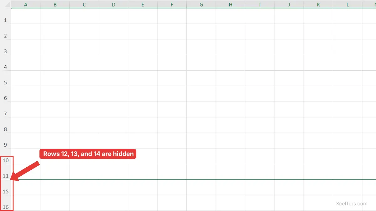
• Row numbers skip, such as 10, 11, 15, and 16, which means rows 12, 13, and 14 are hidden in this example.
• There is a small gap or double line between row numbers.
• Some data appears missing, but formulas still refer to it.
• When you select a large range, Excel may include rows that are not currently visible.

Beginner Tip:
Hidden rows are not deleted. They are still part of the worksheet, and formulas can still use the values inside them.10If you recently followed the previous lesson on how to hide rows in Excel, this is the reverse action. Instead of removing rows from view, you are making them visible again.

Once you know what hidden rows look like, the simplest place to start is restoring one missing row.

How to Unhide Rows in Excel with Right-Click

Right-clicking is one of the easiest ways to unhide rows in Excel because the command appears directly beside the row numbers. This method is especially helpful for beginners because you can clearly select the visible rows around the hidden area before choosing Unhide.

You can use the same right-click method for one hidden row, several adjacent hidden rows, or separate hidden areas. Let’s start with the simplest example: unhiding one row.

How to Unhide a Row in Excel with Right-Click

If only one row is hidden, the fastest method is to select the visible rows around it. This tells Excel exactly where the hidden row is located.

This method is useful when you can clearly see the missing row number. For example, if row numbers jump from 5 to 7, row 6 is hidden.

Follow these steps when one row is missing between two visible rows.

1. Click the row number above the hidden row.
2. Hold Shift and click the row number below the hidden row.
3. Right-click one of the selected row numbers.
4. Click Unhide.

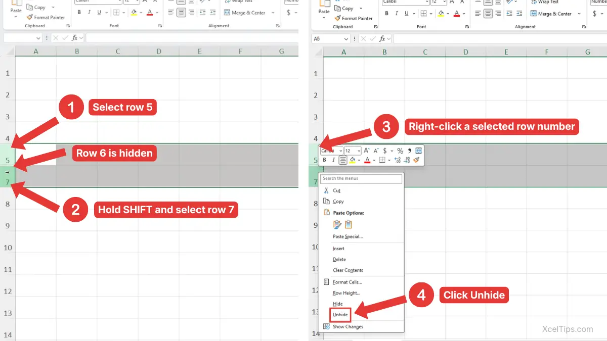
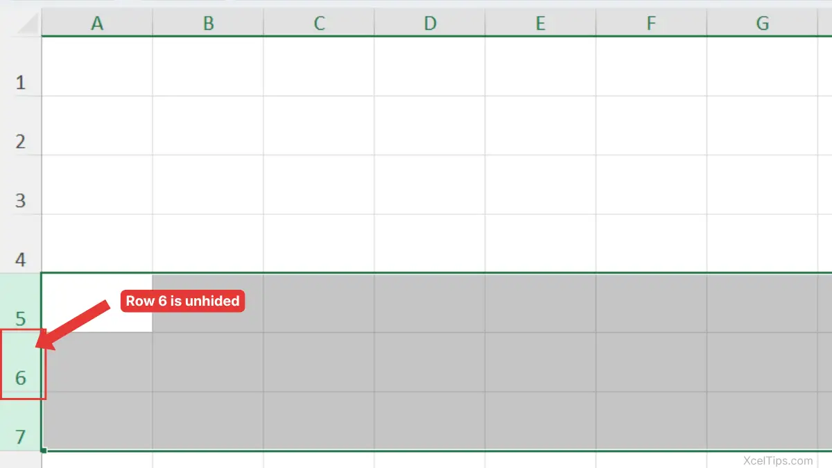
For example, suppose row 6 is hidden. Select rows 5 and 7, right-click the selected row headers, and choose Unhide. Excel brings row 6 back between rows 5 and 7, as shown in the image below.

Beginner Warning:
Do not right-click inside a normal cell if you want to unhide a full row. Right-click the row numbers on the left side instead. This makes sure Excel understands you are working with entire rows.

This is the most common answer to how to unhide a row in Excel because it is simple, visual, and easy to remember.

Once you can restore one hidden row, the next step is learning how to handle several hidden rows at the same time.

How to Unhide Multiple Adjacent Rows with Right-Click

Sometimes more than one row is hidden in the same area. For example, a worksheet may show row 4 and then jump directly to row 10, which means several adjacent rows are hidden between them.

You do not need to unhide each row one by one. To unhide multiple rows in Excel, select the visible row range around the hidden area, then use the same Unhide command.

Use this method when the hidden rows are next to each other.

1. Click the row number above the hidden section.
2. Hold Shift, and click the row number below the hidden section.
3. Right-click one of the selected row numbers.
4. Choose Unhide.

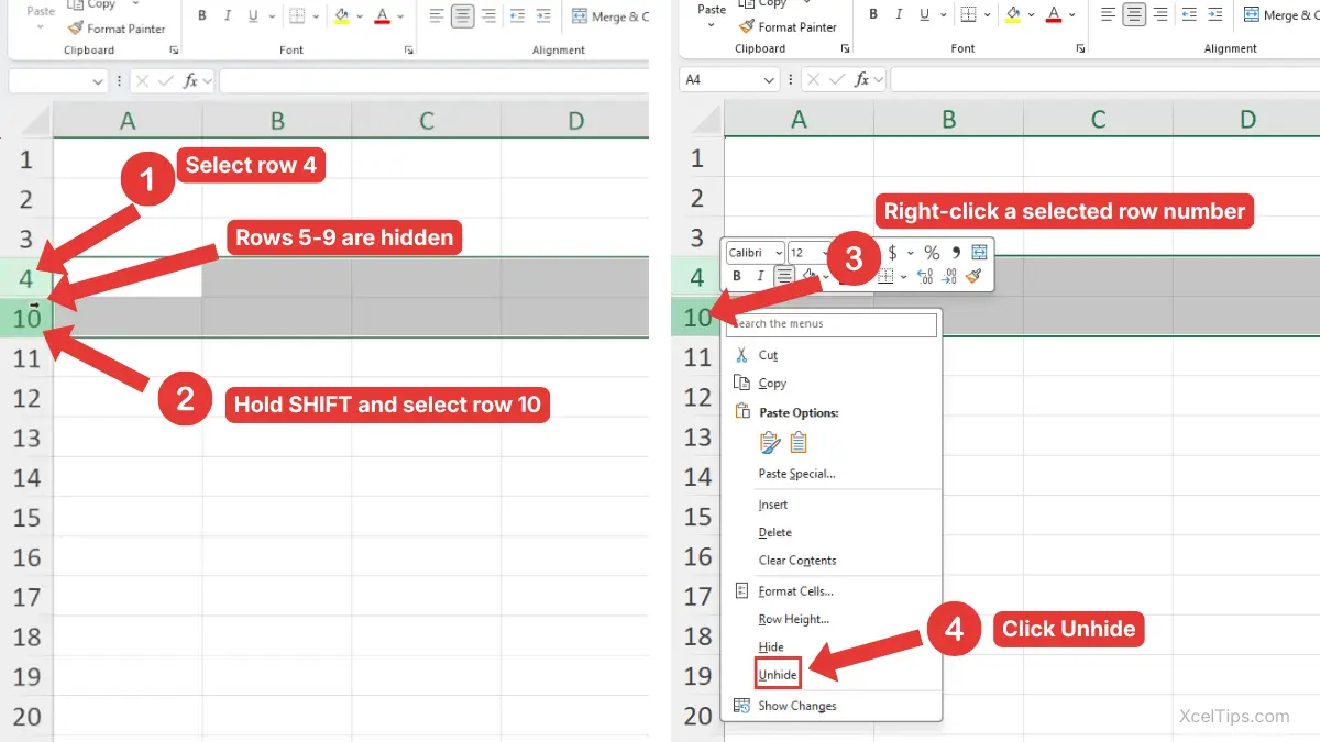
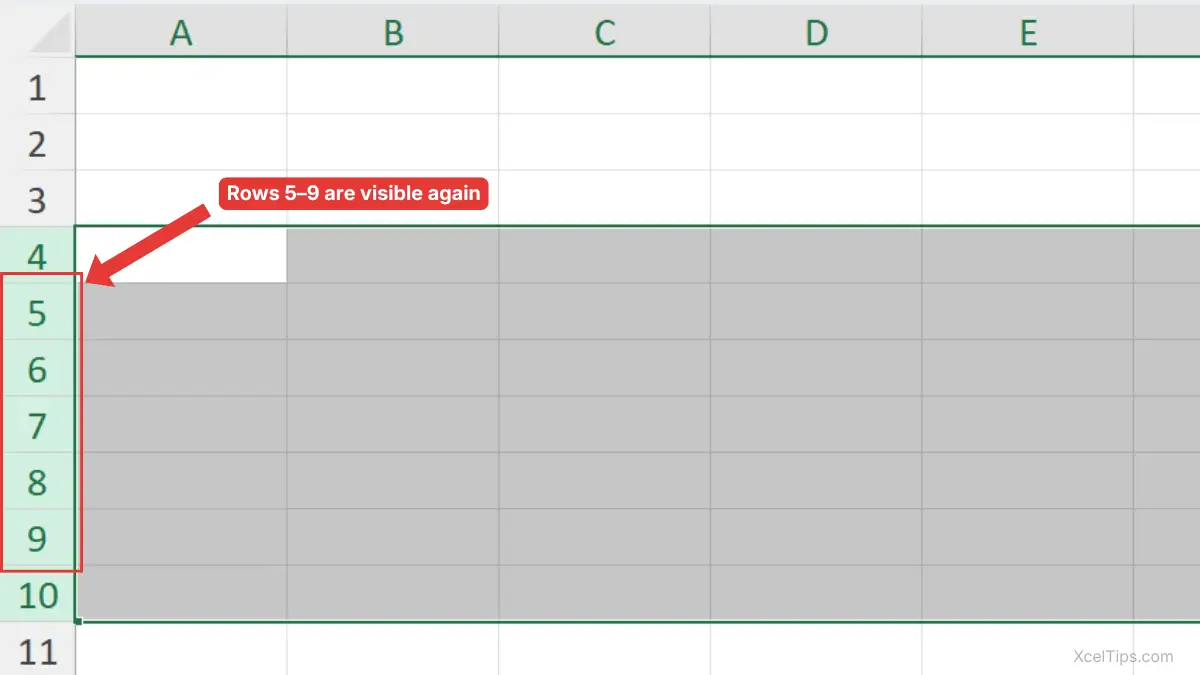
For example, if the worksheet jumps from row 4 to row 10, select rows 4 through 10 by clicking row 4, holding Shift, and clicking row 10. Then right-click the selected row numbers and choose Unhide. Excel will show rows 5, 6, 7, 8, and 9 again, as shown in the image below.

Beginner Tip:
This method is best for adjacent hidden rows. If hidden rows are in separate places, such as rows 5 and 12, unhide each hidden area separately or select the whole worksheet and use Unhide Rows.

If you are not comfortable selecting row numbers yet, you may want to review how to select rows in Excel before practicing this method.

What If Hidden Rows Are Not Next to Each Other?

Sometimes hidden rows are in separate places, such as row 5 and row 12. In that case, the right-click method is still possible, but it is usually easier for beginners to unhide each hidden area separately.

For example, if row 5 is hidden, select rows 4 and 6, right-click, and choose Unhide. Then, if row 12 is hidden, select rows 11 and 13, right-click, and choose Unhide again.

Beginner Tip:
If you are not sure how many hidden rows are in the worksheet, use the Select All method later in this tutorial to unhide all rows at once.

This right-click method works well when you can see where the hidden rows are. But if you prefer using Excel’s Ribbon, there is another beginner-friendly option.

How to Unhide Rows in Excel from the Ribbon

The Ribbon method is useful if you prefer clicking commands from the top of Excel instead of using the right-click menu. It also helps beginners learn where row commands are located in the Excel interface.

This method uses the Format menu on the Home tab. It works after you select the row area that contains hidden rows.

Start by selecting the rows around the hidden area. Then use the command from the Home tab.

1. Select the visible rows above and below the hidden row area.
2. Go to the Home tab.
3. In the Cells group, click Format.
4. Hover over Hide & Unhide.
5. Click Unhide Rows.

Excel will display the hidden rows inside the selected area.

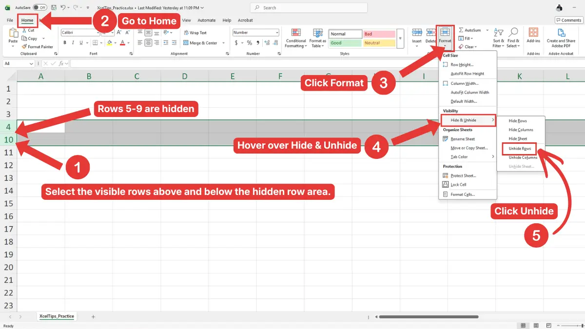
The full path is: Home tab → Cells group → Format → Hide & Unhide → Unhide Rows.

Beginner Warning:
If you click Unhide Rows without selecting the correct row area first, Excel may not bring back the rows you expected. Selection matters.

The Ribbon method is slower than right-clicking for small tasks, but it is very clear and reliable. For repeated work, the keyboard shortcut can be even faster.

Shortcut to Unhide Rows in Excel

Excel also has a keyboard shortcut for unhiding rows. This is helpful when you are working through a worksheet quickly and do not want to open menus.

The shortcut is easy to use, but it still depends on selection. You must select the affected row area before pressing the keys.

After selecting the rows around the hidden area, press Ctrl + Shift + 9.

Here is how to use it:

1. Select the visible rows above and below the hidden row area.
2. Press Ctrl + Shift + 9.
3. Check that the missing rows are now visible.

For example, if row 12 is hidden, select rows 11 and 13, then press Ctrl + Shift + 9. Excel should display row 12 again.

Beginner Tip:
The shortcut works best when entire rows are selected. If the shortcut does not work, try selecting the row numbers first, not just cells inside the worksheet.

Shortcuts are helpful for selected areas, but sometimes you may not know how many rows are hidden. In that case, it is better to unhide everything at once.

How to Unhide All Rows in Excel

If you are not sure where rows are hidden, you can unhide all rows in the worksheet. This is useful when you receive a file from someone else and want to make sure nothing is hidden.

This method selects the whole worksheet first. Then the Unhide command applies to all rows, not just one area.

Method 1: Use the Select All Button

The Select All button is the small triangle at the top-left corner of the worksheet, between the row numbers and column letters.

1. Click the Select All button in the top-left corner of the worksheet.
2. Right-click any visible row number.
3. Click Unhide.

Excel will unhide all hidden rows in the active worksheet.

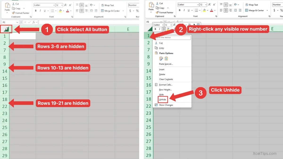
For example, if rows 3–6, 10–13, and 19–21 are hidden in the same worksheet, the Select All method is faster than unhiding each hidden section separately.

Method 2: Use the Ribbon After Selecting the Whole Worksheet

This method uses the same Ribbon command, but applies it to the entire sheet.

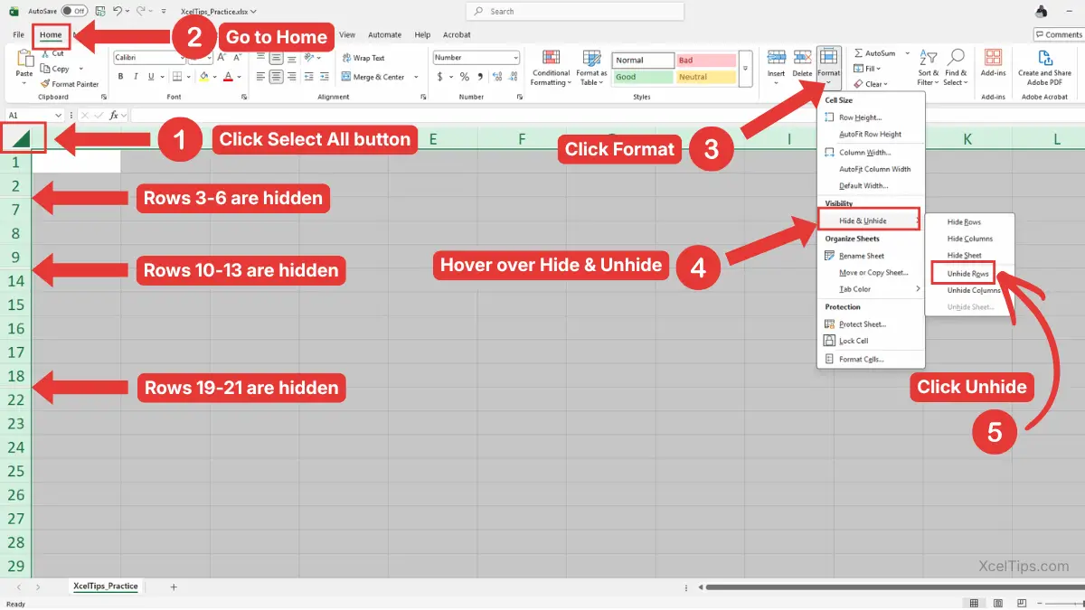
1. Click the Select All button.
2. Go to the Home tab.
3. In the Cells group, click Format.
4. Hover over Hide & Unhide.
5. Click Unhide Rows.

This is a clear answer to how to unhide all rows in Excel because it does not require you to find each hidden section manually.

Beginner Warning:
This only affects the active worksheet. If your workbook has multiple worksheet tabs, repeat the steps on any other sheet where rows may be hidden.

For full-sheet selection basics, you can also review how to select cells and ranges in Excel if that lesson is part of your beginner roadmap.

If the rows still do not appear after using Unhide, something else may be affecting the worksheet.

What to Do If Unhide Rows Does Not Work

Sometimes you choose Unhide, but the missing rows still do not appear. This usually means something else is affecting the worksheet. For beginners, it is important not to panic or assume the data is gone. Check these common causes one at a time.

Check If a Filter Is Hiding Rows

Filtered rows can look similar to hidden rows because row numbers may skip. However, filters are different from normal hidden rows. Look for filter arrows in the header row. If a filter is active, one or more arrows may show a funnel icon. For more detailed tutorials on filter, review how to filter data in Excel.

Check If Row Height Is Very Small

A row may look hidden if its height is set to a very small number. In that case, using Unhide may not always look like it fixed the problem. Set row height to a normal size such as 15 for many default worksheets.

Check If the Sheet Is Protected

If the worksheet is protected, some row commands may be limited. You might not be able to unhide rows until protection is removed. You do not need to learn worksheet protection in detail here. Just look at the Review tab. If you see an option related to unprotecting the sheet, the file may have protection enabled.

For the official Microsoft explanation of this feature, you can also read Microsoft’s guide to hiding and showing rows or columns in Excel.

Once you understand the common problems, it helps to compare the main methods side by side.

Best Method to Use for Different Unhide Row Situations

Different situations call for different methods. A single hidden row is easy to fix with right-click, while a workbook with unknown hidden rows may be easier to fix with Select All.

Use the table below as a quick decision guide when you are not sure which method to choose.

Situation	Best Method	Why It Works Well
One row is hidden	Select rows above and below, then right-click → Unhide	Simple and visual
Several rows are hidden together	Select the surrounding row range, then Unhide	Restores the whole hidden section
Hidden rows are in separate places	Unhide each area separately or use Select All	Avoids confusing non-adjacent selections
Unknown rows are hidden	Select All, then Unhide Rows	Applies to the whole worksheet
You prefer menu commands	Home → Format → Hide & Unhide → Unhide Rows	Easy to follow from the Ribbon
You want a faster method	Select rows, then press Ctrl + Shift + 9	Good for repeated use

This comparison is useful because there is no single best method for every workbook. The best choice depends on what you can see and how much of the sheet may be hidden.

For beginners, the safest method is usually right-clicking the selected row numbers. After that feels comfortable, the shortcut and Ribbon options become easier to use.

Before ending the lesson, practice with a small example so the steps become familiar.

Quick Practice

In a practice worksheet, first hide a row so you can test the Unhide command. Use a blank worksheet or a copy of a simple workbook so you can test the steps safely.

Try this short exercise:

1. Open a worksheet with sample data.
2. Right-click row number 5.
3. Choose Hide.
4. Notice that the row numbers jump from 4 to 6.
5. Select rows 4 and 6.
6. Right-click one of the selected row numbers.
7. Choose Unhide.
8. Confirm that row 5 appears again.

Then try a second practice task:

1. Hide rows 8, 9, and 10.
2. Select rows 7 through 11.
3. Press Ctrl + Shift + 9.
4. Confirm that rows 8, 9, and 10 are visible again.

After practicing the steps, review the main points so you know which method to use next time rows go missing.

Key Takeaways

Unhiding rows is a basic Excel layout skill, but it solves a common beginner problem: missing rows that look like deleted data.

• Hidden rows are still in the worksheet.
• Missing row numbers are a common sign that rows are hidden.
• To unhide one row, select the rows above and below it, then choose Unhide.
• To unhide multiple rows in Excel, select the full surrounding row range.
• To unhide all rows in Excel, select the whole worksheet first.
• The Ribbon path is Home tab → Cells group → Format → Hide & Unhide → Unhide Rows.
• The shortcut to unhide rows is Ctrl + Shift + 9.
• If Unhide does not work, check filters, row height, or worksheet protection.

Finally, here are answers to common beginner questions about hidden rows and the Unhide command.

Frequently Asked Questions (FAQs)

How do I unhide one missing row in Excel?

To unhide one missing row, select the visible row above and the visible row below the hidden row. Then right-click the selected row numbers and choose Unhide.

How do I unhide multiple rows in Excel?

Select the visible row above the hidden section and the visible row below it. Then right-click the selected row numbers and choose Unhide. You can also use Home tab → Format → Hide & Unhide → Unhide Rows.

How do I unhide all rows in Excel at once?

Click the Select All button in the top-left corner of the worksheet, right-click any row number, and choose Unhide. This brings back all normally hidden rows in the active worksheet.

What is the shortcut to unhide rows in Excel?

The shortcut is Ctrl + Shift + 9. Select the row area first, then press the shortcut to show hidden rows.

Why are my rows still missing after I click Unhide?

The rows may be hidden by a filter, set to a very small row height, or restricted by worksheet protection. Check for filter arrows, reset row height, and make sure you have permission to edit the worksheet.

Is unhiding rows the same as deleting or restoring deleted rows?

No. Hidden rows were never deleted. Unhiding simply makes them visible again. Deleted rows are removed from the worksheet and require Undo or file recovery if you need them back.

Once you understand the different methods, unhiding rows becomes a simple worksheet skill you can use whenever data seems to be missing.

Conclusion

Learning How to Unhide Rows in Excel helps you recover missing worksheet information quickly and safely. Whether you need to show one hidden row, multiple hidden rows, row 1, or every hidden row in the sheet, the key is to select the correct row area before using Unhide.

Practice the right-click method first because it is the easiest for beginners. Then try the Ribbon command and Ctrl + Shift + 9 shortcut when you want faster options.

This lesson is part of the Beginner Learning Path, a structured series designed to help you learn Microsoft Excel step by step from the basics.

← Previous Lesson
How to Hide Rows in Excel: Step-by-Step Guide for Beginners

Next Lesson →
How to Hide Columns in Excel Without Deleting Your Data

More Lessons in Module 2 – Working with Data